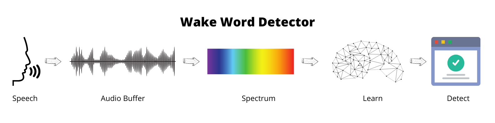
This article will describe the steps required for building a wake word detector.
- Background
- Related Work
- How to train a model from audio files
- Datasets
- How to learn from audio files
- Libraries
- Preparing labeled dataset
- Word Alignment
- Retreive timestamps of words
- Fixing data imbalance
- Adding noise data
- Dataloader
- Transformations
- Model
- Training
- Evaluation
- Inference
- Deploying model in the app
- Demo
- Conclusion
- References
Background
Personal Assistant devices like Google Home, Alexa, and Apple Homepod, will constantly be listening for a specific set of wake words like “Ok, Google” or “Alexa” or “Hey Siri”, and once these sequence of words are detected, it would prompt to the user for subsequent commands and respond to them appropriately. To create a custom wake word detector, which will take audio as input and, once the sequence of words is detected, then prompt the user. The goal is to provide a configurable custom detector so anyone can use it on their application to perform operations once configured wake words are detected.
Related Work
Below two papers heavily influence most of the work discussed here.
- Howl: A Deployed, Open-Source Wake Word Detection System
- Honkling: In-Browser Personalization for Ubiquitous Keyword Spotting
I would highly recommend going through the above papers.
How to train a model from audio files
Below are the steps we will be doing to train a model using audio files
Step 1: Get an audio dataset with transcripts
Step 2: Decide on what wake words to use (mostly 2 to 3 words)
Step 3: Search for these words in dataset transcripts and prepare a positive dataset (that has a wake-word) and negative
dataset (does not have wake-word)
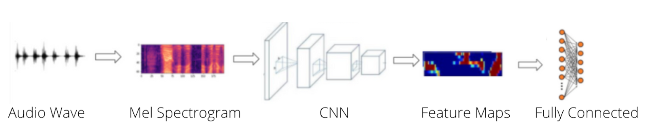
Step 4: Extract audio features by converting them to Mel spectrograms (pictorial representation of audio)
Step 5: Using CNN, train on the above data.
Step 6: Save and test the model
Step 7: Make live inference on the above model.
We will go through each step in detail.
Datasets
First, you need a dataset with transcripts; check Mozilla Common Voice dataset. As of this writing, the dataset size is 73 GB. Download it, and if you extract it, you will see something like the below.
 Directory of D:\GoogleDrive\datasets\cv-corpus-6.1-2020-12-11\en

12/12/2020  06:54 PM    <DIR>          .
12/12/2020  06:54 PM    <DIR>          ..
07/13/2021  02:49 PM    <DIR>          clips
12/17/2020  05:05 PM         3,759,462 dev.tsv
12/17/2020  05:05 PM        44,843,183 invalidated.tsv
12/17/2020  05:05 PM        38,372,321 other.tsv
12/18/2020  01:32 PM           269,523 reported.tsv
12/17/2020  05:05 PM         3,633,900 test.tsv
12/17/2020  05:05 PM       138,386,852 train.tsv
12/17/2020  05:05 PM       285,317,674 validated.tsv
               7 File(s)    514,582,915 bytes
               3 Dir(s)  405,241,425,920 bytes free
clips have all the mp3 files, tsv files have transcripts of these mp3 files. If you open train.tsv using pandas
train_data = pd.read_csv('train.tsv', sep='\t')
train_data.head()
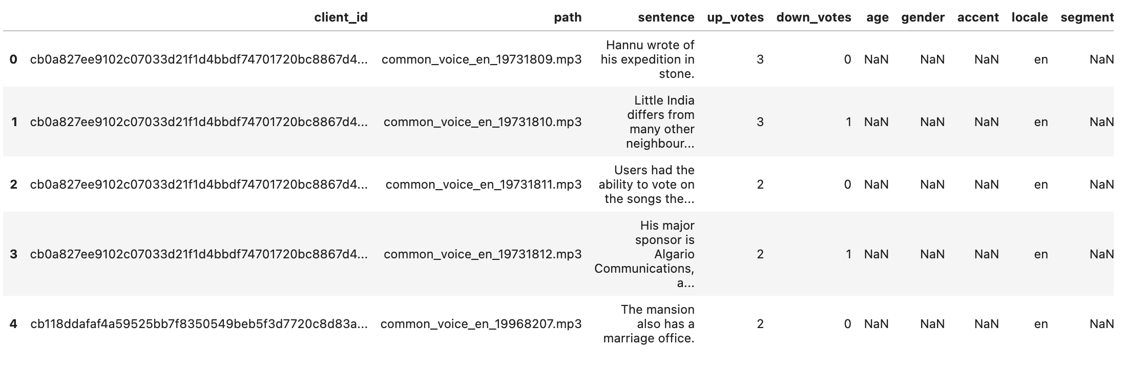
Now, if you play audio file common_voice_en_19731809.mp3 in the clips folder it would say Hannu wrote of his expedition in stone.
For this use case, we only need path and sentence columns.
There are other datasets you can explore please refer
For Noise dataset - Microsoft SNSD (Reddy et al., 2019)
How to learn from audio files
Before going further, we need to know a few concepts. I would strongly recommend going through below articles to learn about how to understand and extract features from audio files.
- Learning from Audio: Wave Forms - Towards Data Science
- Learning from Audio: Fourier Transformations - by mlearnere - Towards ….
- Understanding the Mel Spectrogram - by Leland Roberts - Medium.
Sample rate
The sounds of our voices — are just a sum of many sine and cosine signals. Waves are repeated signals that oscillate and vary in amplitude, depending on their complexity. In the real world, waves are continuous and mechanical — quite different from computers being discrete and digital. So, how do we translate something continuous and mechanical into something discrete and digital? Here is where the sample rate comes in1. The sample rate is the number of points per second used to trace the signal.
Say, for example, the sample rate of the recorded audio is 100; this means that for every recorded second of audio, the computer will place 100 points along the signal to best “trace” the continuous curve. Once all the points are in place, a smooth curve joins them all together for humans to be able to visualize the sound. Since the recorded audio is in terms of amplitude and time, we can intuitively say that the waveform operates in the time domain1.
Simply put, what resolution is to photos, the sample rate is to audio. The high the sample rate, high the quality of the audio.
Usually, 16kHz is enough to get audio features. High-definition audio files or real-time audio streaming will give 44.1 kHz, 48 kHz, then we need to downsample 16kHz.
For example - if you used librosa to load a mp3 audio file
sounddata = librosa.core.load("sample.mp3", sr=16000, mono=True)[0]
If the sample rate is 16000, you will get 16000 data points per second. So here you will get a numpy of size 16000 (filled with floating numbers)
Fourier Transform
Fourier transformation translates the audio from the time domain to the frequency domain.
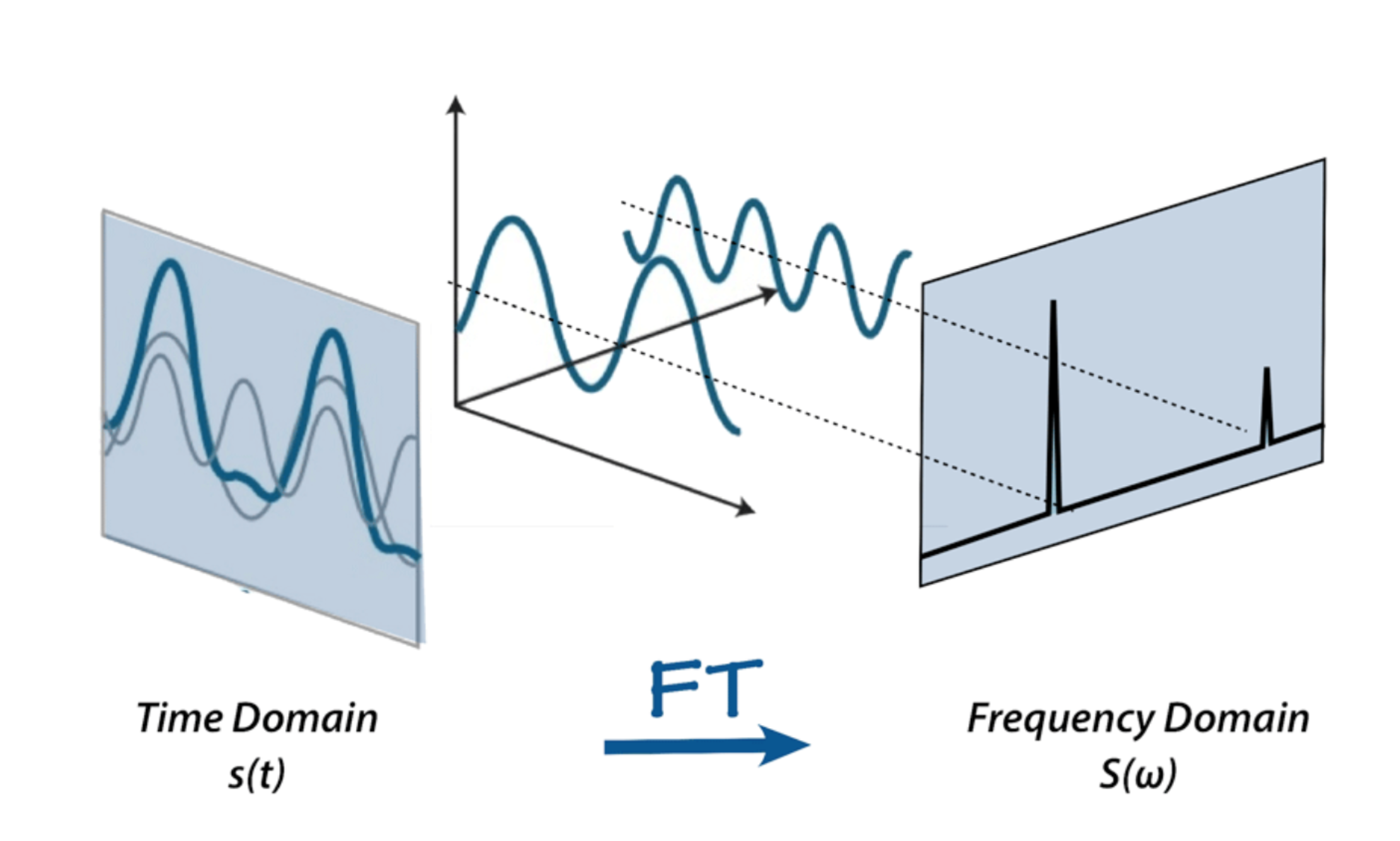
Time domain
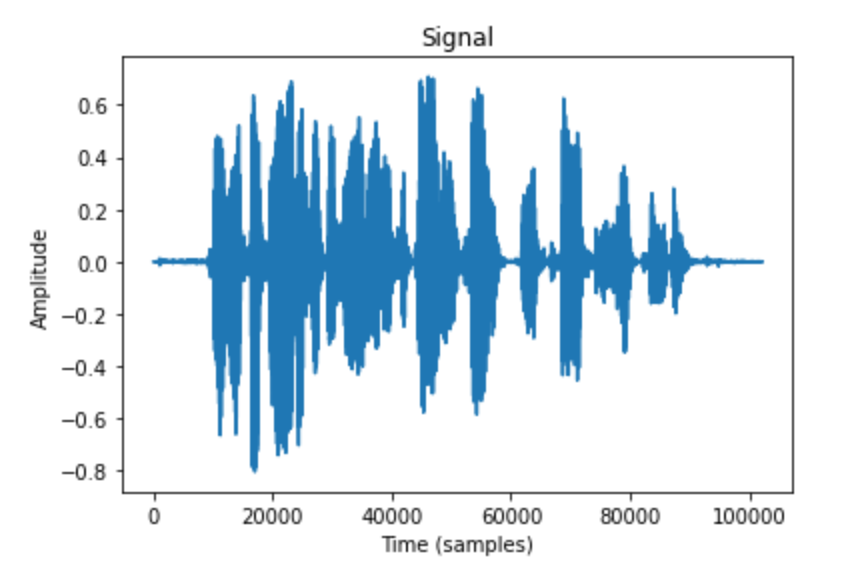
The time domain looks at the signal’s amplitude variation over time, which helps understand its physical shape. To plot this, we need time on the x-axis and amplitude on the y-axis. The shape gives us a good idea of how loud or quiet the sound will be2.
sounddata = librosa.core.load(f"{common_voice_datapath}/clips/common_voice_en_20433916.mp3", sr=sr, mono=True)[0]

# plotting the signal in time series
plt.plot(sounddata)
plt.title('Signal')
plt.xlabel('Time (samples)')
plt.ylabel('Amplitude')
Frequency domain
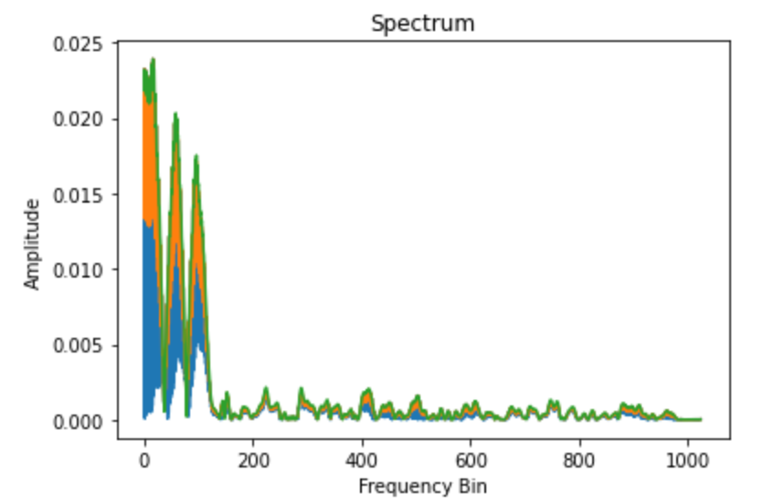
The frequency domain observes the constituent signals our recording is comprised of. By doing this, we can find a sort of “fingerprint” of the sound.To plot this, we need frequency on the x-axis and magnitude on the y-axis.The larger the magnitude, the more important that frequency is. The magnitude is simply the absolute value of our results from the FFT2.
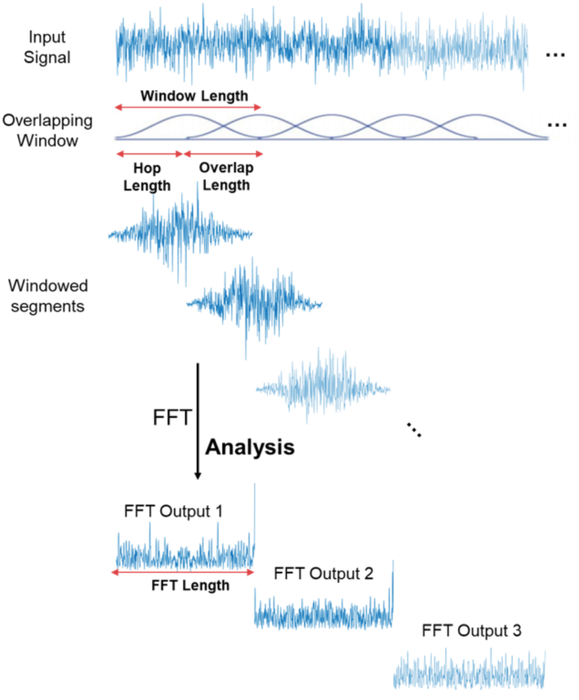
below is how you can calculate FFT for one windowed segment
sounddata = librosa.core.load(f"{common_voice_datapath}/clips/common_voice_en_20433916.mp3", sr=sr, mono=True)[0]

n_fft = 512
ft = np.abs(librosa.stft(sounddata[:n_fft], hop_length = 200))
plt.plot(ft);
plt.title('Spectrum');
plt.xlabel('Frequency Bin');
plt.ylabel('Amplitude');
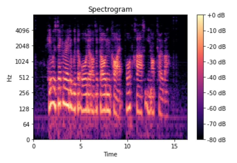
The FFT is computed on overlapping windowed segments of the signal, and we get what is called the spectrogram. You can think of a spectrogram as a bunch of FFTs stacked on top of each other. It is a way to visually represent a signal’s loudness, or amplitude, as it varies over time at different frequencies3.
So to get a spectogram,
# first compute short-time Fourier transform (STFT)
# The y-axis is converted to a log scale
spec = np.abs(librosa.stft(sounddata, hop_length=200))
# the color dimension is converted to decibels (you can think of this as the log scale of the amplitude)
spec = librosa.amplitude_to_db(spec, ref=np.max)

librosa.display.specshow(spec, sr=sr, x_axis='time', y_axis='log');
plt.colorbar(format='%+2.0f dB');
plt.title('Spectrogram');
Mel-Spectrograms
First Spectrogram needs to be computed; for that we need to compute FFT (Fourier transform) The Fourier transform is a mathematical formula that allows us to decompose a signalinto its individual frequencies and the frequency’s amplitude. In other words, it converts the signal from the time domain into the frequency domain. The result is called a spectrum3.
The Mel Scale is a logarithmic transformation of a signal’s frequency The linear audio spectrogram is ideally suited for applications where all frequencies have equal importance, while Mel spectrograms are better suited for applications that need to model human hearing perception. Mel spectrogram data is also suited for use in audio classification applications. The y-axis is converted to a log scale, and the color dimension is converted to decibels3.
So to calculate Mel spectrograms.
# A Mel spectrogram is a spectrogram where the frequencies are converted to the mel scale.
# n_mels -  Mel filters applied which reduces the number of bands to n_mels (typically 32-128)

mel_spect = librosa.feature.melspectrogram(y=sounddata, sr=sr, n_fft=512, hop_length=200)
mel_spect = librosa.power_to_db(mel_spect, ref=np.max)
librosa.display.specshow(mel_spect, y_axis='mel', fmax=8000, x_axis='time');
plt.title('Mel Spectrogram');
plt.colorbar(format='%+2.0f dB');
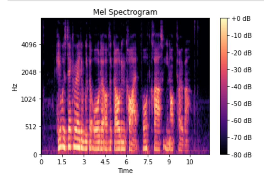
So to summarize, we need to calculate the Mel-spectrograms of all audio files; we will be getting a pictorial representation of the audio file, which we can feed to a CNN to learn the patterns in audio files.
Libraries
Below are the libraries and frameworks we will be using
- Deep Learning Framework - PyTorch
- Audio preprocessing - Librosa, Torchaudio
- Server side Inference - Pyaudio, Websockets, Flask
- Client side Inference - ONNXjs, TensorflowJS, tflite
Preparing labeled dataset
Used Mozilla Common Voice dataset,
- Go through each wake word and check transcripts for match
- If found, then it will be in the positive dataset
- If not found, then it will be in the negative dataset
- Load appropriate mp3 files and trim the silence parts
- save as .wav file and transcript as .lab file
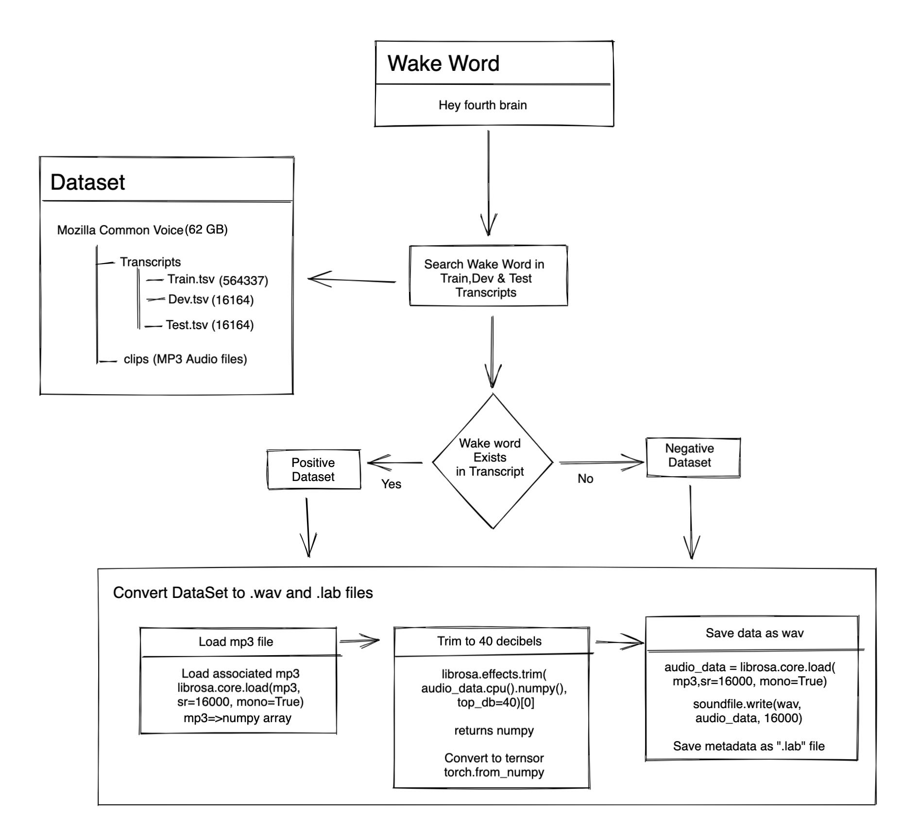
For example, here I am using “Hey Fourth Brain”
wake_words = ["hey", "fourth", "brain"]
wake_words_sequence = ["0", "1", "2"]
Load train, dev and test data
train_data = pd.read_csv("train.tsv", sep="\t")
dev_data = pd.read_csv("dev.tsv", sep="\t")
test_data = pd.read_csv("test.tsv", sep="\t")
Use below regex pattern, find transcripts that contain any wake words.
wake_word_seq_map = dict(zip(wake_words, wake_words_sequence))
regex_pattern = r"\b(?:{})\b".format("|".join(map(re.escape, wake_words)))
pattern = re.compile(regex_pattern, flags=re.IGNORECASE)


def wake_words_search(pattern, word):
    try:
        return bool(pattern.search(word))
    except TypeError:
        return False

positive_train_data = train_data[[wake_words_search(pattern, sentence) for sentence in train_data["sentence"]]]
positive_dev_data = dev_data[[wake_words_search(pattern, sentence) for sentence in dev_data["sentence"]]]
positive_test_data = test_data[[wake_words_search(pattern, sentence) for sentence in test_data["sentence"]]]

negative_train_data = train_data[[not wake_words_search(pattern, sentence) for sentence in train_data["sentence"]]]
negative_dev_data = dev_data[[not wake_words_search(pattern, sentence) for sentence in dev_data["sentence"]]]
negative_test_data = test_data[[not wake_words_search(pattern, sentence) for sentence in test_data["sentence"]]]
You will get a large negative dataset, so sample to 1%
# trim negative data size to 1%
negative_data_percent = 1
negative_train_data = negative_train_data.sample(
    math.floor(negative_train_data.shape[0] * (negative_data_percent / 100))
)
negative_dev_data = negative_dev_data.sample(math.floor(negative_dev_data.shape[0] * (negative_data_percent / 100)))
negative_test_data = negative_test_data.sample(math.floor(negative_test_data.shape[0] * (negative_data_percent / 100)))
Save as .wav and .lab file, this format is required for word alignment step.
def save_wav_lab(path, filename, sentence, decibels=40):
    # load file
    sounddata = librosa.core.load(f"{common_voice_datapath}/clips/{filename}", sr=sr, mono=True)[0]
    # trim
    sounddata = librosa.effects.trim(sounddata, top_db=decibels)[0]
    # save as wav file
    soundfile.write(f"{wake_word_datapath}{path}/{filename.split('.')[0]}.wav", sounddata, sr)
    # write lab file
    with open(f"{wake_word_datapath}{path}/{filename.split('.')[0]}.lab", "w", encoding="utf-8") as f:
        f.write(sentence)
Word Alignment
We need to know where the wake word is used in the audio.
For example - if in the audio file positive/audio/common_voice_en_20812859.wav, the utterance is of The fourth candidate is awarded a two-year term.
then what timestamps in the audio file, the word fourth uttered?
How to find these timestamps, for this we use word alignment software like Montreal Forced Alignment
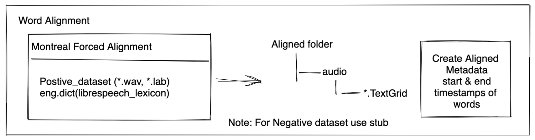
For positive dataset, used Montreal Forced Alignment to get timestamps of each word in audio.
Download the stable version
wget https://github.com/MontrealCorpusTools/Montreal-Forced-Aligner/releases/download/v1.0.1/montreal-forced-aligner_linux.tar.gz
tar -xf montreal-forced-aligner_linux.tar.gz
rm montreal-forced-aligner_linux.tar.gz
Download the Librispeech Lexicon dictionary
wget https://www.openslr.org/resources/11/librispeech-lexicon.txt
Known issues in MFA
# known mfa issue https://github.com/MontrealCorpusTools/Montreal-Forced-Aligner/issues/109
cp montreal-forced-aligner/lib/libpython3.6m.so.1.0 montreal-forced-aligner/lib/libpython3.6m.so
cd montreal-forced-aligner/lib/thirdparty/bin && rm libopenblas.so.0 && ln -s ../../libopenblasp-r0-8dca6697.3.0.dev.so libopenblas.so.0
Creating aligned data
montreal-forced-aligner\bin\mfa_align -q positive\audio librispeech-lexicon.txt montreal-forced-aligner\pretrained_models\english.zip aligned_data
Note that we only need run alignment on the positive dataset. Above should create a bunch of TextGrid files; if you try to open it should be like below
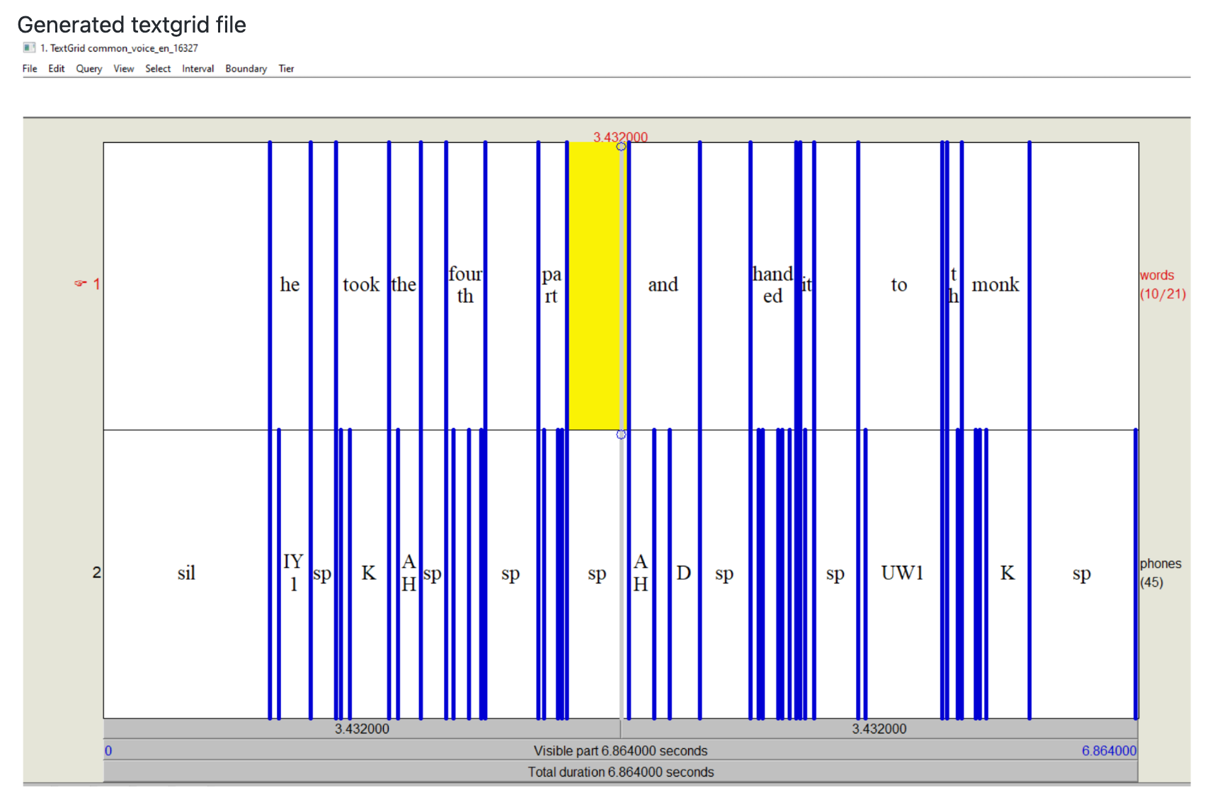
Retreive timestamps of words
Now you can read those Textgrid files to get word timestamps and duration.
def get_timestamps(path):
  filename = path.split('/')[-1].split('.')[0]
  filepath = f'aligned_data/audio/{filename}.TextGrid'
  words_timestamps = {}
  if os.path.exists(filepath):
    tg = textgrid.TextGrid.fromFile(filepath)
    for tg_intvl in range(len(tg[0])):
      word = tg[0][tg_intvl].mark
      if word:
        words_timestamps[word] = {'start': tg[0][tg_intvl].minTime, 'end':  tg[0][tg_intvl].maxTime}
  return words_timestamps

def get_duration(path):
   sounddata = librosa.core.load(path, sr=sr, mono=True)[0]
   return sounddata.size / sr * 1000 # ms
Apply above methods on positive data
positive_train_data = pd.read_csv('positive/train.csv')
positive_dev_data = pd.read_csv('positive/dev.csv')
positive_test_data = pd.read_csv('positive/test.csv')

positive_train_data['path'] = positive_train_data['path'].apply(lambda x: 'positive/audio/'+x.split('.')[0]+'.wav')
positive_dev_data['path'] = positive_dev_data['path'].apply(lambda x: 'positive/audio/'+x.split('.')[0]+'.wav')
positive_test_data['path'] = positive_test_data['path'].apply(lambda x: 'positive/audio/'+x.split('.')[0]+'.wav')

positive_train_data['timestamps'] = positive_train_data['path'].progress_apply(get_timestamps)
positive_dev_data['timestamps'] = positive_dev_data['path'].progress_apply(get_timestamps)
positive_test_data['timestamps'] = positive_test_data['path'].progress_apply(get_timestamps)

positive_train_data['duration'] = positive_train_data['path'].progress_apply(get_duration)
positive_dev_data['duration'] = positive_dev_data['path'].progress_apply(get_duration)
positive_test_data['duration'] = positive_test_data['path'].progress_apply(get_duration)
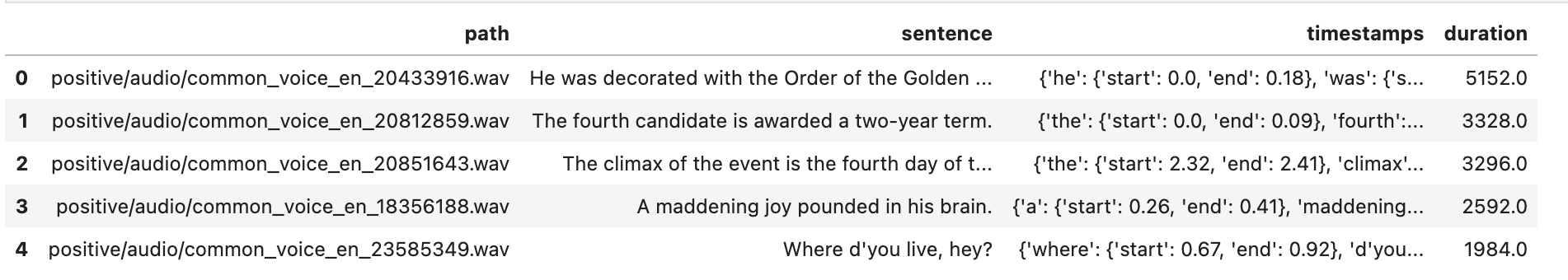
Positive train data would look like below
positive_train_data.head()
Do the same for negative dataset, however since we have not run MFA on negative dataset, you will get empty.
negative_train_data = pd.read_csv('negative/train.csv')
negative_dev_data = pd.read_csv('negative/dev.csv')
negative_test_data = pd.read_csv('negative/test.csv')

negative_train_data['path'] = negative_train_data['path'].apply(lambda x: 'negative/audio/'+x.split('.')[0]+'.wav')
negative_dev_data['path'] = negative_dev_data['path'].apply(lambda x: 'negative/audio/'+x.split('.')[0]+'.wav')
negative_test_data['path'] = negative_test_data['path'].apply(lambda x: 'negative/audio/'+x.split('.')[0]+'.wav')

negative_train_data['timestamps'] = negative_train_data['path'].progress_apply(get_timestamps)
negative_dev_data['timestamps'] = negative_dev_data['path'].progress_apply(get_timestamps)
negative_test_data['timestamps'] = negative_test_data['path'].progress_apply(get_timestamps)

negative_train_data['duration'] = negative_train_data['path'].progress_apply(get_duration)
negative_dev_data['duration'] = negative_dev_data['path'].progress_apply(get_duration)
negative_test_data['duration'] = negative_test_data['path'].progress_apply(get_duration)
Negative train data would look like below
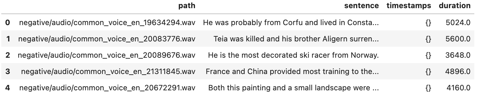
Fixing data imbalance
You can check how much each wake word spread on the dataset you created above.
# checking pattern spread on train_ds
hey_pattern = re.compile(r'\bhey\b', flags=re.IGNORECASE)
fourth_pattern = re.compile(r'\bfourth\b', flags=re.IGNORECASE)
brain_pattern = re.compile(r'\bbrain\b', flags=re.IGNORECASE)

print(f"Total hey word {(train_ds[[wake_words_search(hey_pattern, sentence) for sentence in train_ds['sentence']]].size/train_ds.size) * 100} %")
print(f"Total fourth word {(train_ds[[wake_words_search(fourth_pattern, sentence) for sentence in train_ds['sentence']]].size/train_ds.size) * 100} %")
print(f"Total brain word {(train_ds[[wake_words_search(brain_pattern, sentence) for sentence in train_ds['sentence']]].size/train_ds.size) * 100
The above should give a result like the below. The spread is not equal among the dataset.
Total hey word 0.9193357058125742 %
Total fourth word 11.728944246737841 %
Total brain word 3.855278766310795 %
To fix this, you can generate additional data using Google TTS.
generated_data = 'generated'
Path(f"{wake_word_datapath}/{generated_data}").mkdir(parents=True, exist_ok=True)

os.environ["GOOGLE_APPLICATION_CREDENTIALS"]="your_service_acc.json"

from google.cloud import texttospeech
# Instantiates a client
client = texttospeech.TextToSpeechClient()

import time
def generate_voices(word):
  Path(f"{wake_word_datapath}/{generated_data}/{word}").mkdir(parents=True, exist_ok=True)
  # Set the text input to be synthesized
  synthesis_input = texttospeech.SynthesisInput(text=word)
  # Performs the list voices request
  voices = client.list_voices()
  # Get english voices
  en_voices =  [voice.name for voice in voices.voices if voice.name.split("-")[0] == 'en']
  speaking_rates = np.arange(0.25, 4.25, 0.25).tolist()
  pitches = np.arange(-10.0, 10.0, 2).tolist()
  file_count = 0
  start = time.time()

  for voi in en_voices:
    for sp_rate in speaking_rates:
      for pit in pitches:
        file_name = f'{wake_word_datapath}/{generated_data}/{word}/{voi}_{sp_rate}_{pit}.wav'
        voice = texttospeech.VoiceSelectionParams(language_code=voi[:5], name=voi)
        # Select the type of audio file you want returned
        audio_config = texttospeech.AudioConfig(
            # format of the audio byte stream.
            audio_encoding=texttospeech.AudioEncoding.LINEAR16,

            #Speaking rate/speed, in the range [0.25, 4.0]. 1.0 is the normal native speed
            speaking_rate=sp_rate,

            #Speaking pitch, in the range [-20.0, 20.0]. 20 means increase 20 semitones from the original pitch. -20 means decrease 20 semitones from the original pitch.
            pitch=pit # [-10, -5, 0, 5, 10]
        )
        response = client.synthesize_speech(
          request={"input": synthesis_input, "voice": voice, "audio_config": audio_config}
        )
        # The response's audio_content is binary.
        with open(file_name, "wb") as out:
            out.write(response.audio_content)
            file_count+=1
        if file_count%100 == 0:
          end = time.time()
          print(f"generated {file_count} files in {end-start} seconds")
Using generate_voices method, generate for each wake word by varying speaking rate and speaking pitch, we can
generate 7K samples for each wake word.
Now we can create csv file with path and sentence.
for word in wake_words:
  d = {}
  d['path'] = [f"{generated_data}/{word}/{file_name}" for file_name in os.listdir(f"{wake_word_datapath}/{generated_data}/{word}")]
  d['sentence'] = [word] * len(d['path'])
  pd.DataFrame(data=d).to_csv(f"{generated_data}/{word}.csv", index=False)
Split generated data into train, dev and test
word_cols = {'path' : [], 'sentence': []}
train, dev, test = pd.DataFrame(word_cols), pd.DataFrame(word_cols), pd.DataFrame(word_cols)
for word in wake_words:
  word_df = pd.read_csv(f"{generated_data}/{word}.csv")
  tra, val, te =  np.split(word_df.sample(frac=1, random_state=42),  [int(.6*len(word_df)), int(.8*len(word_df))])
  train = pd.concat([train , tra]).sample(frac=1).reset_index(drop=True)
  dev = pd.concat([dev , val]).sample(frac=1).reset_index(drop=True)
  test = pd.concat([test , te]).sample(frac=1).reset_index(drop=True)

train.to_csv(f"{generated_data}/train.csv", index=False)
dev.to_csv(f"{generated_data}/dev.csv", index=False)
test.to_csv(f"{generated_data}/test.csv", index=False)
Since we already know what generated audio files have, we don’t need to run MFA. So we can add some dummy values.
# add dummy values for these columns for generated data
train['timestamps'] = ''
train['duration'] = ''

dev['timestamps'] = ''
dev['duration'] = ''

test['timestamps'] = ''
test['duration'] = ''
Now combine generated data with actual data and check the distribution.
train_ds = pd.concat([train_ds , train]).sample(frac=1).reset_index(drop=True)
dev_ds = pd.concat([dev_ds , dev]).sample(frac=1).reset_index(drop=True)
test_ds = pd.concat([test_ds , test]).sample(frac=1).reset_index(drop=True)

# now verify how much data we have for train set
print(f"Total hey word {(train_ds[[wake_words_search(hey_pattern, sentence) for sentence in train_ds['sentence']]].size/train_ds.size) * 100} %")
print(f"Total fourth word {(train_ds[[wake_words_search(fourth_pattern, sentence) for sentence in train_ds['sentence']]].size/train_ds.size) * 100} %")
print(f"Total brain word {(train_ds[[wake_words_search(brain_pattern, sentence) for sentence in train_ds['sentence']]].size/train_ds.size) * 100} %")
That should be looking something like the below.
Total hey word 22.398959583833534 %
Total fourth word 26.04541816726691 %
Total brain word 23.389355742296917 %
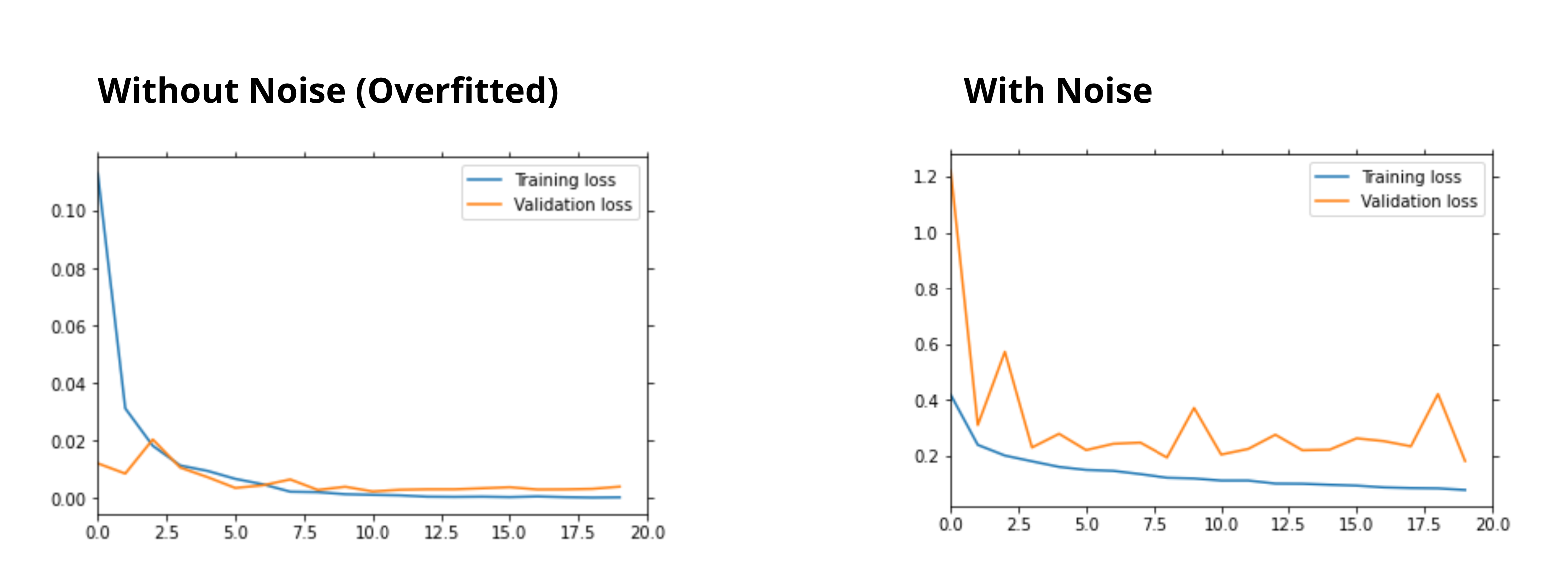
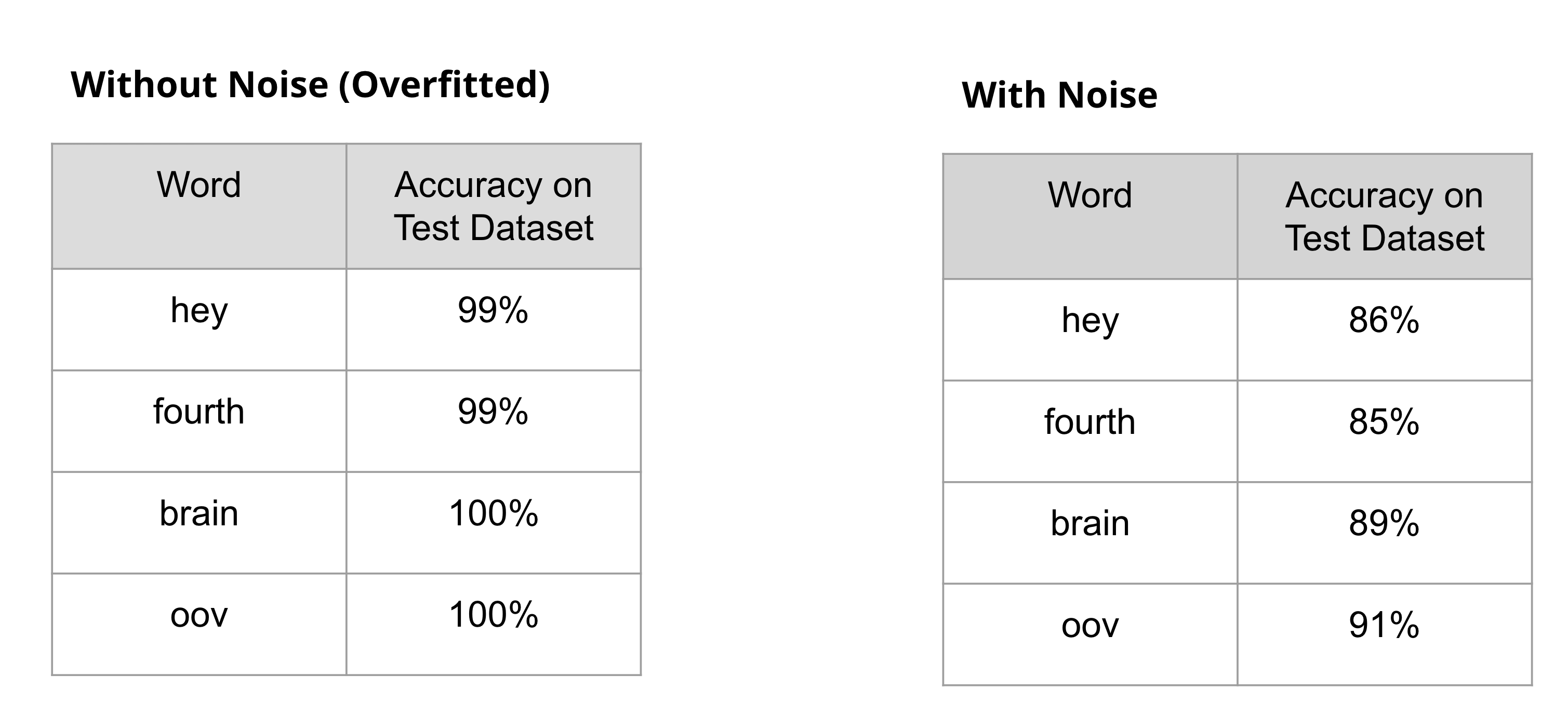
Adding noise data
For wake word detection to work correctly, we need to add noise; in the real world, there would be a lot of background noise which will be fed to the model, so the model should be aware of that noise. Without noise, model will be overfitting.
You can noise dataset from Microsoft Scalable Noisy Speech Dataset.
We are interested in two folders, noise_train and noise_test.
Load noise dataset.
%%bash
find noise/noise_train/ -name "*.wav" | wc -l
find noise/noise_test/ -name "*.wav" | wc -l
You can listen to one noise sample
noise_sample = librosa.core.load('noise/noise_train/AirConditioner_1.wav', sr=sr, mono=True)[0]
Audio(noise_sample, rate=sr)
Now lets take a clean sample
clean_sample = librosa.core.load('generated/brain/en-AU-Standard-A_0.75_0.0.wav', sr=sr, mono=True)[0]
Audio(clean_sample, rate=sr)
For example - if the clean_sample size is 12560.
Then you can take 12560 data points from the noise sample.
Now, if you mix clean and noise samples together like below
Audio(clean_sample + noise_sample[:12560], rate=sr)
hear noise sample is added 100%, but you can bring the noise down like below
noise_level = 0.2
Audio((1 - noise_level) * clean_sample +  noise_level * noise_sample[:12560], rate=sr)
In the above, we mixed 80% of the clean sample with 20% of the noise sample.
Dataloader
Now we have all the data required to train the model. Now we need to create a data loader that can be used during training.
We will be using window size as 750ms and sample rate as 16K so that the max length would be int(window_size_ms/1000 * sr).
and that would come to 12000.
- Load the audio file
- Compute labels
- if it is generated file, then we know the label
- if it is from MCV, then we have timestamps to know where precisely to trim to get the word
- If the audio length > max length (12000), then trim randomly either at the start or end of the audio
- If audio length < max length (12000), then pad zeros at the start or end of the audio
- Add noise ranging from 10 to 50% randomly.
The full code will be like the below.
key_pattern = re.compile("\'(?P<k>[^ ]+)\'")
def compute_labels(metadata, audio_data):
  label = len(wake_words) # by default negative label

  # if it is generated data then
  if metadata['sentence'].lower() in wake_words:
    label = int(wake_word_seq_map[metadata['sentence'].lower()])
  else:
    # if the sentence has one wakeword get the label and end timestamp
    for word in metadata['sentence'].lower().split():
      wake_word_found = False
      word = re.sub('\W+', '', word)
      if word in wake_words:
        wake_word_found = True
        break

    if wake_word_found:
      label = int(wake_word_seq_map[word])
      if word in  metadata['timestamps']:
        timestamps = metadata['timestamps']
        if type(timestamps) == str:
          timestamps = json.loads(key_pattern.sub(r'"\g<k>"', timestamps))
        word_ts = timestamps[word]
        audio_start_idx = int((word_ts['start'] * 1000) * sr / 1000)
        audio_end_idx = int((word_ts['end'] * 1000) * sr / 1000)
        audio_data = audio_data[audio_start_idx:audio_end_idx]
      else: # if there are issues with word alignment, we might not get ts
        label = len(wake_words)  # mark them for negative

  return label, audio_data

class AudioCollator(object):
  def __init__(self, noise_set=None):
    self.noise_set = noise_set

  def __call__(self, batch):
    batch_tensor = {}
    window_size_ms = 750
    max_length = int(window_size_ms/1000 * sr)
    audio_tensors = []
    labels = []
    for sample in batch:
      # get audio_data in tensor format
      audio_data = librosa.core.load(sample['path'], sr=sr, mono=True)[0]
      # get the label and its audio
      label, audio_data = compute_labels(sample, audio_data)
      audio_data_length = audio_data.size / sr * 1000 #ms

      # below is to make sure that we always got length of 12000
      # i.e 750 ms with sr 16000
      # trim to max_length
      if audio_data_length > window_size_ms:
        # randomly trim either at start and end
        if random.random() < 0.5:
          audio_data = audio_data[:max_length]
        else:
          audio_data = audio_data[audio_data.size-max_length:]

      # pad with zeros
      if audio_data_length < window_size_ms:
        # randomly either append or prepend
        if random.random() < 0.5:
          audio_data = np.append(audio_data, np.zeros(int(max_length - audio_data.size)))
        else:
          audio_data = np.append(np.zeros(int(max_length - audio_data.size)), audio_data)

      # Add noise
      if self.noise_set:
        noise_level =  random.randint(1, 5)/10 # 10 to 50%
        noise_sample = librosa.core.load(self.noise_set[random.randint(0,len(self.noise_set)-1)], sr=sr, mono=True)[0]
        # randomly select first or last seq of noise
        if random.random() < 0.5:
          audio_data = (1 - noise_level) * audio_data +  noise_level * noise_sample[:max_length]
        else:
          audio_data = (1 - noise_level) * audio_data +  noise_level * noise_sample[-max_length:]

      audio_tensors.append(torch.from_numpy(audio_data))
      labels.append(label)

    batch_tensor = {
        'audio': torch.stack(audio_tensors),
        'labels': torch.tensor(labels)
    }

    return batch_tensor
Now we can use the above methods to create dataloder
batch_size = 16
num_workers = 0

train_audio_collator = AudioCollator(noise_set=noise_train)
train_dl = tud.DataLoader(train_ds.to_dict(orient='records'),
                  batch_size=batch_size,
                  drop_last=True,
                  shuffle=True,
                  num_workers=num_workers,
                  collate_fn=train_audio_collator)

dev_audio_collator = AudioCollator(noise_set=noise_dev)
dev_dl = tud.DataLoader(dev_ds.to_dict(orient='records'),
                  batch_size=batch_size,
                  num_workers=num_workers,
                  collate_fn=dev_audio_collator)

test_audio_collator = AudioCollator(noise_set=noise_test)
test_dl = tud.DataLoader(test_ds.to_dict(orient='records'),
                  batch_size=batch_size,
                  num_workers=num_workers,
                  collate_fn=test_audio_collator)
Transformations
MelSpectrogram
As mentioned above the input to our model would be log mel spectrograms. We already have the raw audio data in dataloaders, we need to transform them to log mel spectrograms. Pytorch audio already has torchaudio.transforms.MelSpectrogram to transform to mel spectrograms,
num_mels = 40 # https://en.wikipedia.org/wiki/Mel_scale
num_fft = 512 # window length - Fast Fourier Transform
hop_length = 200  # making hops of size hop_length each time to sample the next window
def audio_transform(audio_data):
  # Transformations
  # Mel-scale spectrogram is a combination of Spectrogram and mel scale conversion
  # 1. compute FFT - for each window to transform from time domain to frequency domain
  # 2. Generate Mel Scale - Take entire freq spectrum & seperate to n_mels evenly spaced
  #    frequencies. (not by distance on freq domain but distance as it is heard by human ear)
  # 3. Generate Spectrogram - For each window, decompose the magnitude of the signal
  #    into its components, corresponding to the frequencies in the mel scale.
  mel_spectrogram  = MelSpectrogram(n_mels=num_mels,
                                    sample_rate=sr,
                                    n_fft=num_fft,
                                    hop_length=hop_length,
                                    norm='slaney')
  mel_spectrogram.to(device)
  log_mels = mel_spectrogram(audio_data.float()).add_(1e-7).log_().contiguous()
  # returns (channel, n_mels, time)
  return log_mels.to(device)
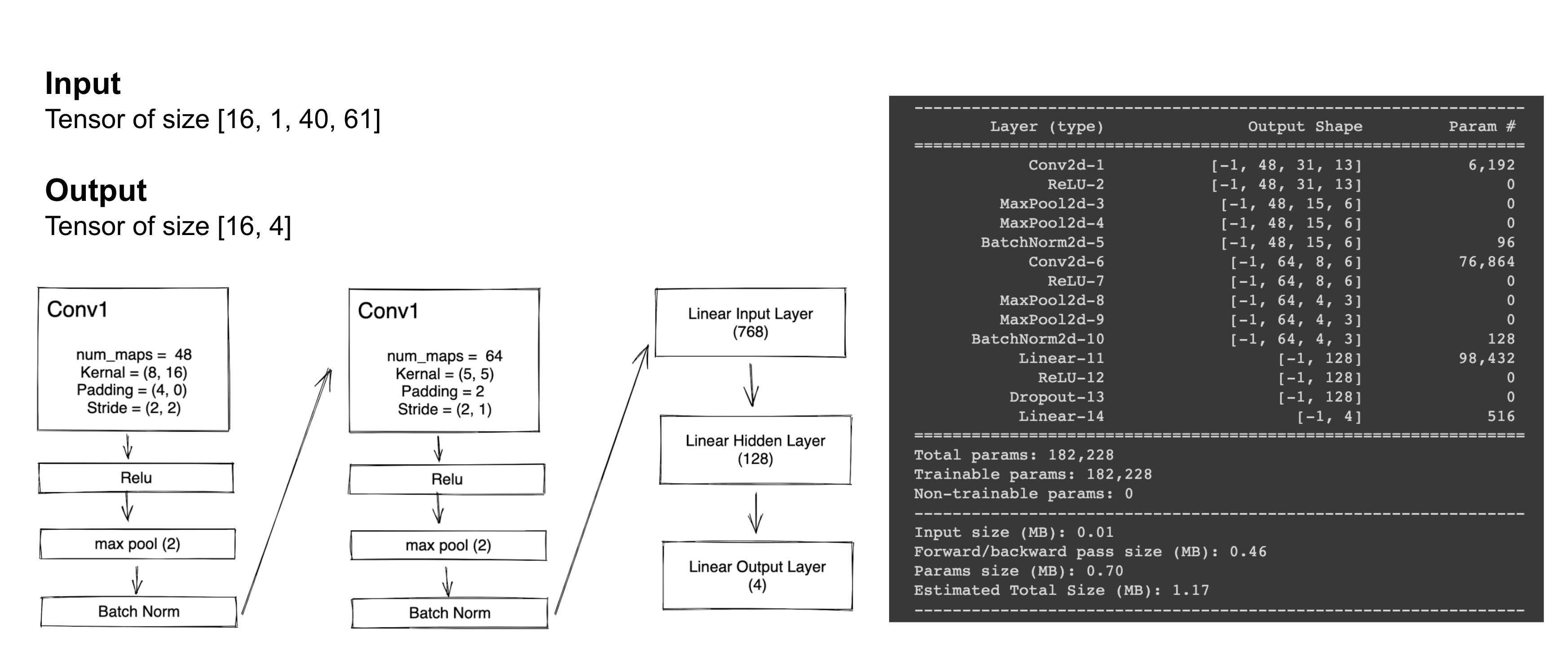
With sample rate = 16000, number of fft’s = 512, hop length = 200, number of mel bands 40 for the sample of 750 ms, we know we get 12000 data points; we said we want 40 mel bands, each with length (12000/200 + 1) = 61, so we would end up with a 40 x 61 matrix. When you pass the audio file to the above method, you will get a tensor of shape (1, 40, 61)
Now we need a CNN model which can take this tensor and train on it.
Zero Mean Unit Variance
We can further normalize the above values using ZMUV.
from typing import Iterable
class ZmuvTransform(nn.Module):
    def __init__(self):
        super().__init__()
        self.register_buffer('total', torch.zeros(1))
        self.register_buffer('mean', torch.zeros(1))
        self.register_buffer('mean2', torch.zeros(1))

    def update(self, data, mask=None):
        with torch.no_grad():
            if mask is not None:
                data = data * mask
                mask_size = mask.sum().item()
            else:
                mask_size = data.numel()
            self.mean = (data.sum() + self.mean * self.total) / (self.total + mask_size)
            self.mean2 = ((data ** 2).sum() + self.mean2 * self.total) / (self.total + mask_size)
            self.total += mask_size

    def initialize(self, iterable: Iterable[torch.Tensor]):
        for ex in iterable:
            self.update(ex)

    @property
    def std(self):
        return (self.mean2 - self.mean ** 2).sqrt()

    def forward(self, x):
        return (x - self.mean) / self.std
We take 1 batch of train dataset, calculate Mean and Standard deviation
zmuv_audio_collator = AudioCollator()
zmuv_dl = tud.DataLoader(train_ds.to_dict(orient='records'),
                  batch_size=1,
                  num_workers=num_workers,
                  collate_fn=zmuv_audio_collator)

zmuv_transform = ZmuvTransform().to(device)
if Path("zmuv.pt.bin").exists():
    zmuv_transform.load_state_dict(torch.load(str("zmuv.pt.bin")))
else:
  for idx, batch in enumerate(tqdm(zmuv_dl, desc="Constructing ZMUV")):
    zmuv_transform.update(batch['audio'].to(device))
  print(dict(zmuv_mean=zmuv_transform.mean, zmuv_std=zmuv_transform.std))
  torch.save(zmuv_transform.state_dict(), str("zmuv.pt.bin"))

print(f"Mean is {zmuv_transform.mean.item():0.6f}")
print(f"Standard Deviation is {zmuv_transform.std.item():0.6f}")
Below is the Mean and Standard Deviation
Mean is 0.000016
Standard Deviation is 0.072771
So after calculating the Mel spectrogram, each value will be subtracted with the above mean and divided by the standard deviation to normalize.
Model
We will be using 2 conv layers and 2 linear layers.
    def __init__(self, num_labels, num_maps1, num_maps2, num_hidden_input, hidden_size):
        super(CNN, self).__init__()
        conv0 = nn.Conv2d(1, num_maps1, (8, 16), padding=(4, 0), stride=(2, 2), bias=True)
        pool = nn.MaxPool2d(2)
        conv1 = nn.Conv2d(num_maps1, num_maps2, (5, 5), padding=2, stride=(2, 1), bias=True)
        self.num_hidden_input = num_hidden_input
        self.encoder1 = nn.Sequential(conv0,
                                      nn.ReLU(),
                                      pool,
                                      nn.BatchNorm2d(num_maps1, affine=True))
        self.encoder2 = nn.Sequential(conv1,
                                      nn.ReLU(),
                                      pool,
                                      nn.BatchNorm2d(num_maps2, affine=True))
        self.output = nn.Sequential(nn.Linear(num_hidden_input, hidden_size),
                                    nn.ReLU(),
                                    nn.Dropout(0.1),
                                    nn.Linear(hidden_size, num_labels))
With below parameters
num_labels = len(wake_words) + 1 # oov
num_maps1  = 48
num_maps2  = 64
num_hidden_input =  768
hidden_size = 128
model = CNN(num_labels, num_maps1, num_maps2, num_hidden_input, hidden_size)
So our model summary for 1x40x61 would be like below - summary(model, input_size=(1,40,61))
Training
Below are the hyper parameters that’s used.
learning_rate = 0.001
weight_decay = 0.0001 # Weight regularization
lr_decay = 0.95

criterion = nn.CrossEntropyLoss()
params = list(filter(lambda x: x.requires_grad, model.parameters()))
optimizer = AdamW(params, learning_rate, weight_decay=weight_decay)
During training,
- First, we pass the audio data to get the Mel spectrogram and
- then pass through zmuv_transform to get normalized values and
- we change the dimension from (batch, channels, n_mels, time) to (batch, channels, time, n_mels)
- We pass through 2 Conv layers
- Next, flatten and pass through 2 linear layers.
    def forward(self, x):
        x = x.permute(0, 1, 3, 2)  # change to (time, n_mels)
        # pass through first conv layer
        x1 = self.encoder1(x)
        # pass through second conv layer
        x2 = self.encoder2(x1)
        # flattening - keep first dim batch same, flatten last 3 dims
        x = x2.view(x2.size(0), -1)
        return x
for epoch in mb:
  x.append(epoch)
  # Evaluate
  model.train()
  total_loss = torch.Tensor([0.0]).to(device)
  #pbar = tqdm(train_dl, total=len(train_dl), position=0, desc="Training", leave=True)
  for batch in progress_bar(train_dl, parent=mb):
    audio_data = batch['audio'].to(device)
    labels = batch['labels'].to(device)
    # get mel spectograms
    mel_audio_data = audio_transform(audio_data)
    # do zmuv transform
    mel_audio_data = zmuv_transform(mel_audio_data)
    predicted_scores = model(mel_audio_data.unsqueeze(1))
    # get loss
    loss = criterion(predicted_scores, labels)

    optimizer.zero_grad()
    model.zero_grad()

    # backward propagation
    loss.backward()
    optimizer.step()

    with torch.no_grad():
        total_loss += loss

  for group in optimizer.param_groups:
    group["lr"] *= lr_decay

  mean = total_loss / len(train_dl)
  training_losses.append(mean.cpu())
Finally save the model - torch.save(model.state_dict(), 'model.pt')
Evaluation
Now do the evaluation using the test dataset
# iterate over test data
pbar = tqdm(test_dl, total=len(test_dl), position=0, desc="Testing", leave=True)
for batch in pbar:
# move tensors to GPU if CUDA is available
audio_data = batch['audio'].to(device)
labels = batch['labels'].to(device)
# forward pass: compute predicted outputs by passing inputs to the model
mel_audio_data = audio_transform(audio_data)
# do zmuv transform
mel_audio_data = zmuv_transform(mel_audio_data)
output = model(mel_audio_data.unsqueeze(1))
# calculate the batch loss
loss = criterion(output, labels)
# update test loss
test_loss += loss.item()*audio_data.size(0)
# convert output probabilities to predicted class
_, pred = torch.max(output, 1)
# compare predictions to true label
correct_tensor = pred.eq(labels.data.view_as(pred))
correct = np.squeeze(correct_tensor.numpy()) if not train_on_gpu else np.squeeze(correct_tensor.cpu().numpy())
# calculate test accuracy for each object class
for i in range(labels.shape[0]):
label = labels.data[i]
class_correct[label.long()] += correct[i].item()
class_total[label.long()] += 1
# for confusion matrix
actual.append(classes[labels.data[i].long().item()])
predictions.append(classes[pred.data[i].item()])
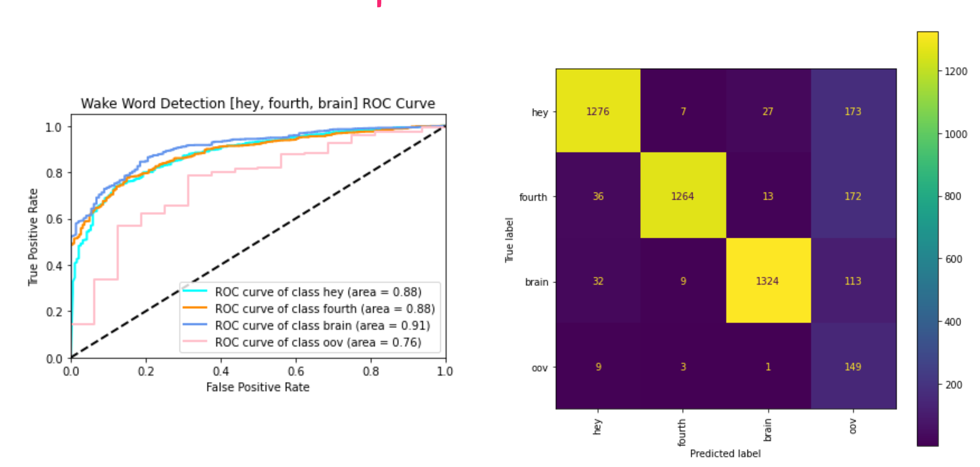
# plot confusion matrix
cm = confusion_matrix(actual, predictions, labels=classes)
print(classification_report(actual, predictions))
cmp = ConfusionMatrixDisplay(cm, classes)
fig, ax = plt.subplots(figsize=(8,8))
cmp.plot(ax=ax, xticks_rotation='vertical')
Inference
Now you can use pyaudio to stream audio and make inferences on live stream; for every 750ms, collect samples and feed them to model to make the inference.
model.eval()

classes = wake_words[:]
# oov
classes.append("oov")

audio_float_size = 32767
p = pyaudio.PyAudio()

CHUNK = 500
FORMAT = pyaudio.paInt16
CHANNELS = 1
RATE = sr
RECORD_MILLI_SECONDS = 750

stream = p.open(format=FORMAT,
                channels=CHANNELS,
                rate=RATE,
                input=True,
                frames_per_buffer=CHUNK)

print("* listening .. ")

inference_track = []
target_state = 0

while True:
  no_of_frames = 4

  #import pdb;pdb.set_trace()
  batch = []
  for frame in range(no_of_frames):
    frames = []
    for i in range(0, int(RATE / CHUNK * RECORD_MILLI_SECONDS/1000)):
        data = stream.read(CHUNK)
        frames.append(data)
    audio_data = np.frombuffer( b''.join(frames), dtype=np.int16).astype(np.float) / audio_float_size
    inp = torch.from_numpy(audio_data).float().to(device)
    batch.append(inp)

  audio_tensors = torch.stack(batch)

  #sav_temp_wav(frames)
  mel_audio_data = audio_transform(audio_tensors)
  mel_audio_data = zmuv_transform(mel_audio_data)
  scores = model(mel_audio_data.unsqueeze(1))
  scores = F.softmax(scores, -1).squeeze(1)  # [no_of_frames x num_labels]
  #import pdb;pdb.set_trace()
  for score in scores:
    preds = score.cpu().detach().numpy()
    preds = preds / preds.sum()
    # print([f"{x:.3f}" for x in preds.tolist()])
    pred_idx = np.argmax(preds)
    pred_word = classes[pred_idx]
    #print(f"predicted label {pred_idx} - {pred_word}")
    label = wake_words[target_state]
    if pred_word == label:
      target_state += 1 # go to next label
      inference_track.append(pred_word)
      print(inference_track)
      if inference_track == wake_words:
        print(f"Wake word {' '.join(inference_track)} detected")
        target_state = 0
        inference_track = []
        break
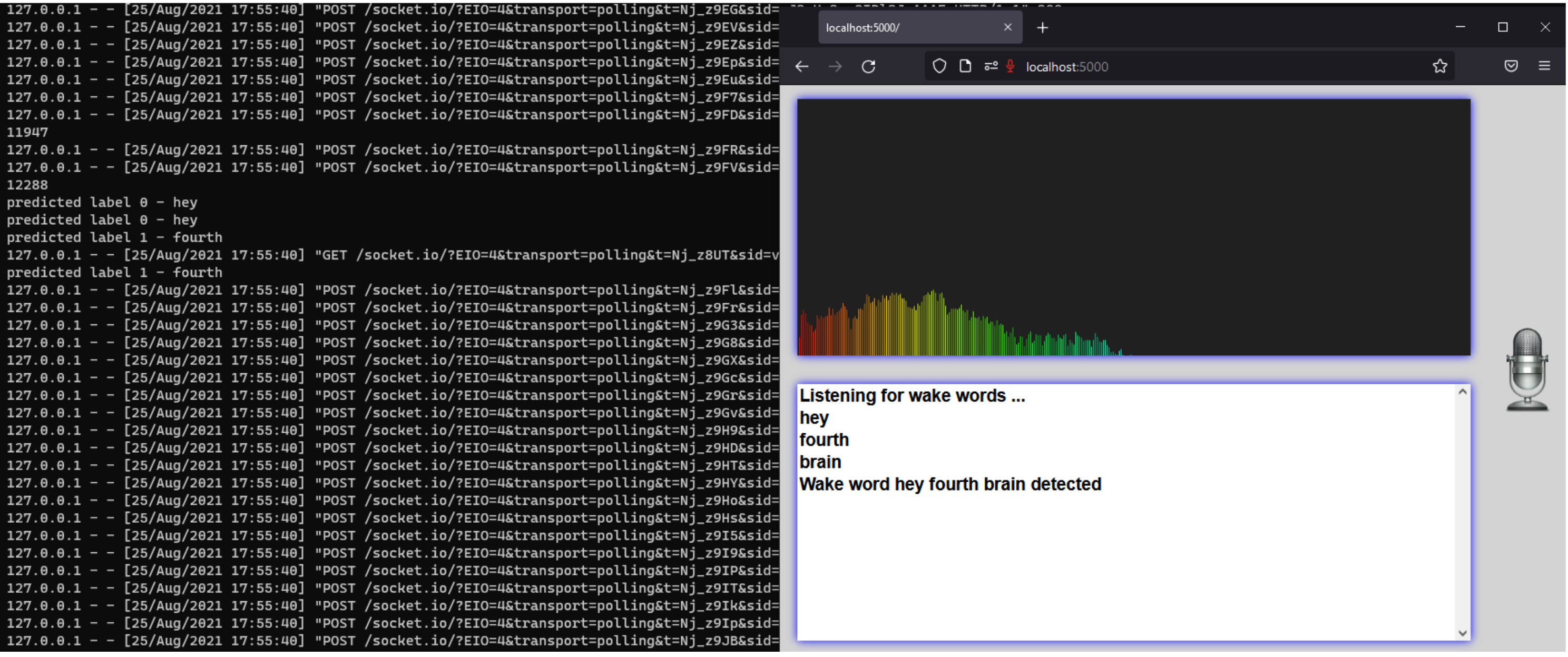
Below is how the wake word sequence will be detected.
['hey']
['hey', 'fourth']
['hey', 'fourth', 'brain']
Wake word hey fourth brain detected
Deploying model in the app
Usually, if you are deploying in any IoT device or raspberry pi and if that device has a microphone and speaker, pyaudio should work, but let’s say if you want to deploy on an application where it will be accessed through the browser, then there are a couple of ways to do it
Using web sockets
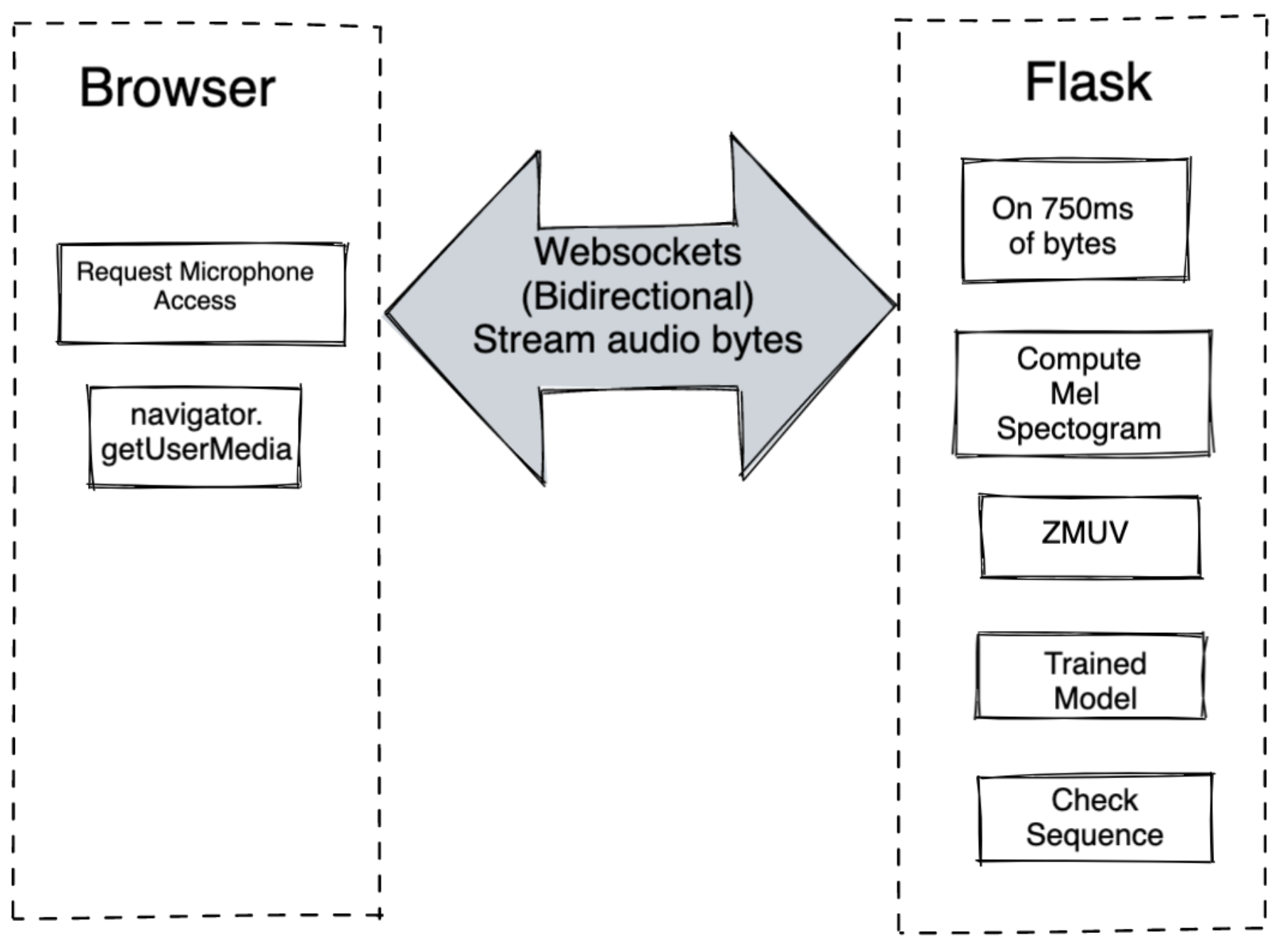
- Using Flask Socketio at server level to capture audio buffer from client.
- At Client, use socket.io at client level to send audio buffer through socket connection.
- Capture audio buffer using getUserMedia, convert to array buffer and stream to server.
- Inference will happen at server, after n batches of 750ms window
- If sequence detected, send detected prompt to client.
- Server Code - application.py
- Client Code - main.js
- To run this locally
  cd server
  python -m venv .venv
  pip install -r requirements.txt
  FLASK_ENV=development FLASK_APP=application.py .venv/bin/flask run --port 8011
- Use Dockerfile & Dockerrun.aws.json to containerize the app and deploy to AWS Elastic BeanStalk
- Elastic Beanstalk initialize app
eb init -p docker-19.03.13-ce wakebot-app --region us-west-2 - Create Elastic Beanstalk instance
eb create wakebot-app --instance_type t2.large --max-instances 1 - Disadvantage of the above method might be privacy, since we are sending the audio buffer to the server for inference
Using ONNX
- Use Pytorch onnx to convert pytorch model to onnx model
- Pytorch to onnx convert code - convert_to_onnx.py
- Once converted, onnx model can be used at client side to do inference
- Client side, used onnx.js to do inference at client level
- Capture audio buffer at client using getUserMedia, convert to array buffer
- Used fft.js to compute Fourier Transform
- Used methods from Meganta.js audio utils to compute audio transformations like Mel spectrograms
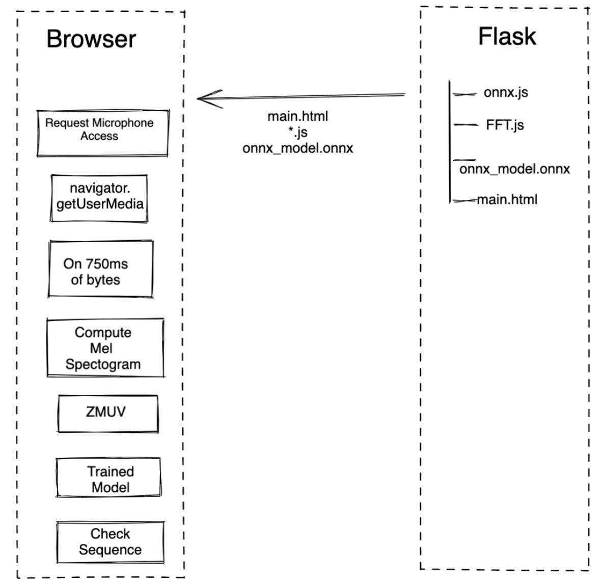
- Below is the comparision of client side vs server side audio transformations
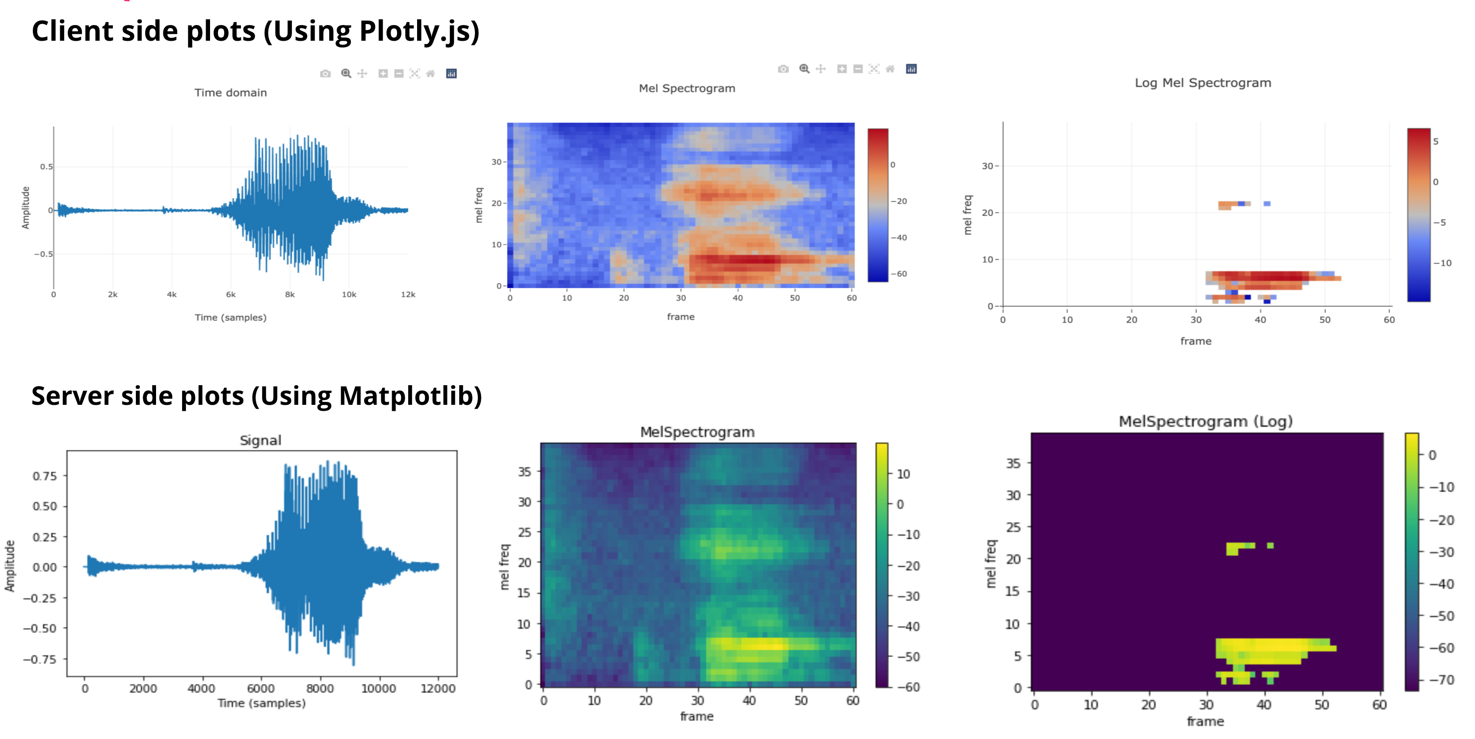
- Client side code - main.js
- To run locally
cd standalone python -m venv .venv pip install -r requirements.txt FLASK_ENV=development FLASK_APP=application.py .venv/bin/flask run --port 8011 - To deploy to AWS Elastic Beanstalk, first initialize app
eb init -p python-3.7 wakebot-std-app --region us-west-2 - Create Elastic Beanstalk instance
eb create wakebot-std-app --instance_type t2.large --max-instances 1 - Refer standalone_onnx for the client version without flask; you can deploy on any static server. You can also deploy to IPFS
- Recent version will show plots and audio buffer for each wake word which model was inferred for; click on the wake word button to know what buffer was inferred for that word.
Using tensorflowjs
- Use onnx-tensorflow to convert onnx model to tensorflow model
- onnx to tensorflow convert code - convert_onnx_to_tf.py
onnx_model = onnx.load("onnx_model.onnx") # load onnx model tf_rep = prepare(onnx_model) # prepare tf representation # Input nodes to the model print("inputs:", tf_rep.inputs) # Output nodes from the model print("outputs:", tf_rep.outputs) # All nodes in the model print("tensor_dict:") print(tf_rep.tensor_dict) tf_rep.export_graph("hey_fourth_brain") # export the model - Verify the model using the below command
python .venv/lib/python3.8/site-packages/tensorflow/python/tools/saved_model_cli.py show --dir hey_fourth_brain --allOutput
MetaGraphDef with tag-set: 'serve' contains the following SignatureDefs: signature_def['__saved_model_init_op']: The given SavedModel SignatureDef contains the following input(s): The given SavedModel SignatureDef contains the following output(s): outputs['__saved_model_init_op'] tensor_info: dtype: DT_INVALID shape: unknown_rank name: NoOp Method name is: signature_def['serving_default']: The given SavedModel SignatureDef contains the following input(s): inputs['input'] tensor_info: dtype: DT_FLOAT shape: (-1, 1, 40, 61) name: serving_default_input:0 The given SavedModel SignatureDef contains the following output(s): outputs['output'] tensor_info: dtype: DT_FLOAT shape: (-1, 4) name: PartitionedCall:0 Method name is: tensorflow/serving/predict Defined Functions: Function Name: '__call__' Named Argument #1 input Function Name: 'gen_tensor_dict' - Refer onnx_to_tf for generated files
- Test converted model using test_tf.py
- Used tensorflowjs[wizard] to convert
savedModelto web model(.venv) (base) ➜ onnx_to_tf git:(main) ✗ tensorflowjs_wizard Welcome to TensorFlow.js Converter. ? Please provide the path of model file or the directory that contains model files. If you are converting TFHub module please provide the URL. hey_fourth_brain ? What is your input model format? (auto-detected format is marked with *) Tensorflow Saved Model * ? What is tags for the saved model? serve ? What is signature name of the model? signature name: serving_default ? Do you want to compress the model? (this will decrease the model precision.) No compression (Higher accuracy) ? Please enter shard size (in bytes) of the weight files? 4194304 ? Do you want to skip op validation? This will allow conversion of unsupported ops, you can implement them as custom ops in tfjs-converter. No ? Do you want to strip debug ops? This will improve model execution performance. Yes ? Do you want to enable Control Flow V2 ops? This will improve branch and loop execution performance. Yes ? Do you want to provide metadata? Provide your own metadata in the form: metadata_key:path/metadata.json Separate multiple metadata by comma. ? Which directory do you want to save the converted model in? web_model converter command generated: tensorflowjs_converter --control_flow_v2=True --input_format=tf_saved_model --metadata= --saved_model_tags=serve --signature_name=serving_default --strip_debug_ops=True --weight_shard_size_bytes=4194304 hey_fourth_brain web_model ... File(s) generated by conversion: Filename Size(bytes) group1-shard1of1.bin 729244 model.json 28812 Total size: 758056 - Once the above step is done, copy the files to the web application
Example -
├── index.html └── static └── audio ├── audio_utils.js ├── fft.js ├── main.js ├── mic128.png ├── model │ ├── group1-shard1of1.bin │ └── model.json ├── prompt.mp3 └── styles.css - Client-side used tfjs to load model and do inference
- Loading the TensorFlow model
let tfModel; async function loadModel() { tfModel = await tf.loadGraphModel('static/audio/model/model.json'); } loadModel() - Do inference using above model
  let outputTensor = tf.tidy(() => {
  let inputTensor = tf.tensor(dataProcessed, [batch, 1, MEL_SPEC_BINS, dataProcessed.length/(batch * MEL_SPEC_BINS)], 'float32');
  let outputTensor = tfModel.predict(inputTensor);
      return outputTensor
  });
  let outputData = await outputTensor.data();
Using tflite
- Once the tensorflow model is created, it can be converted to tflite, using the below code
model = tf.saved_model.load("hey_fourth_brain") input_shape = [1, 1, 40, 61] func = tf.function(model).get_concrete_function(input=tf.TensorSpec(shape=input_shape, dtype=np.float32, name="input")) converter = tf.lite.TFLiteConverter.from_concrete_functions([func]) tflite_model = converter.convert() open("hey_fourth_brain.tflite", "wb").write(tflite_model) - Note:
tf.lite.TFLiteConverter.from_saved_model("hey_fourth_brain")did not work, as it was throwingconv.cc:349 input->dims->data[3] != filter->dims->data[3] (0 != 1)on inference, so used above method. - copy the tflite model to the web application
- Used tflite js to load model and do inference
- Loading tflite model
  let tfliteModel;
  async function loadModel() {
      tfliteModel = await tflite.loadTFLiteModel('static/audio/hey_fourth_brain.tflite');
  }
  loadModel()
Demo
- For a live demo
- ONNX version -https://wake-onnx.netlify.app
- Tensorflow js version - https://wake-tf.netlify.app/
- Tensorflow lite js version - https://wake-tflite.netlify.app/
- Allow microphone to capture audio
- Model is trained on
hey fourth brain- once those words are detected is the sequence; for each detected wake word, a play button to listen to what sound was used to detect that word, and what Mel spectrograms are used will be listed.
Conclusion
In this article, we have gone through how to extract audio features from audio and train model and detect wake words using end-to-end examples with source code. Go through wake_word_detection.ipynb jupyter notebook for a complete walk-through of what is discussed in this article. I hope this helps.
– RC
References
-
Learning from Audio: Wave Forms - Towards Data Science. https://towardsdatascience.com/learning-from-audio-wave-forms-46fc6f87e016 ↩ ↩2
-
Learning from Audio: Fourier Transformations - by mlearnere - Towards …. https://towardsdatascience.com/learning-from-audio-fourier-transformations-f000124675ee ↩ ↩2
-
Understanding the Mel Spectrogram - by Leland Roberts - Medium. https://medium.com/analytics-vidhya/understanding-the-mel-spectrogram-fca2afa2ce53 ↩ ↩2 ↩3

Comments